Weighted Clustering with Minimum-Maximum Cluster Sizes, Greenfield Analysis

This post provides a center of gravity based algorithm for a greenfield analysis. Algorithm is based on k-means clustering enhanced with optimization.

Greenfield Analysis

Greenfield analysis is a quick way to identify optimal distribution center locations for a given demand network. The analysis answers the following questions:

• Where should distribution centers be geographically located to minimize cost?
• Which customers will be supplied from each distribution center?

Problem

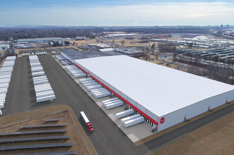
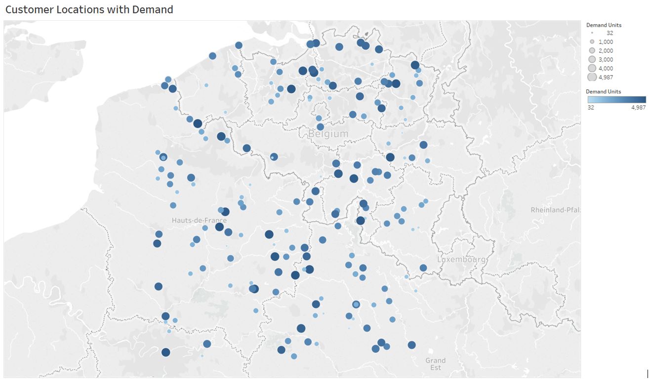
We consider a network of customers where demand for each customer is satisfied by a distribution center. Figure 1 shows the customer locations and corresponding annual demand.

Figure 1: Customer demand map

It is assumed that any location can be selected for a distribution center location.

We answer the following questions as a result of the analysis:

• How many distribution centers are required?
• Where should each distribution center be located?
• How customers should be allocated to the distribution centers?

Algorithm

Algorithm is based on the center of gravity approach and selects the each distribution center locations such that total weighted distance to customers is minimized.

We first provide the following definitions related to the distribution network.

Let $n$ be the total number of distribution centers. Let $D=\{1,\dots,n\}$ be the set of distribution centers and $\hat{D}_i$ be the set of customers allocated to the distribution center $i\in D$. Each distribution center $i\in D$ has latitude and longitude, $\phi^{d}_i$ and $\lambda^{d}_i$, respectively. Let $\alpha_i$ be the maximum distance covered by the center $i \in D$. Let $u^{-}_i$ and $u^{+}_i$ be the minimum and maximum number of customers can be allocated to center $i \in D$, respectively.

Let $C$ be the set of customers. Similar to distribution centers, each customer $j\in C$ has latitude and longitude, $\phi^{c}_j$ and $\lambda^{c}_j$, respectively. Let $d_j$ be the total demand for the customer $j\in C$.

Let $\Delta_k$ be the total weighted distance at iteration $k$.

Let $a_{ij}$ be the distance from the center $i \in D$ to customer $j \in C$. Each $a_{ij}$ is defined using the Haversine distance formula which calculates the shortest distance between two points on a sphere using their latitudes and longitudes measured along the surface. You can find more detailed explanation at the Wikipedia page.

The algorithm consists of the following steps:

Step 0: Set $k=0$. For given $D=\{1, \dots, n\}$, create $\hat{D}_i$ randomly. Let $\Delta_0 = \sum_{i\in D}\sum_{j\in \hat{D}_i}d_ja_{ij}$.

Step 1: Set $k=k+1$. For each $i \in D$, $j \in C$, $u^{-}_i$, $u^{+}_i$, $\alpha_i$, and $a_{ij}$, run a binary allocation model to determine $\hat{D}_i$. Let $\Delta_k = \sum_{i\in D}\sum_{j\in \hat{D}_i}d_ja_{ij}$.

Step 2: If $\Delta_k \ge \Delta_{k-1}$, then stop. Otherwise, set $\phi^{d}_i = \frac{\sum_{j \in \hat{D}_i} \phi^{c}_j}{|D_i|}$ and $\lambda^{d}_i = \frac{\sum_{j \in \hat{D}_i} \lambda^{c}_j}{|D_i|}$ $\forall i\in D$. Repeat Steps 1-2 until $\Delta_k \ge \Delta_{k-1}$.

Allocation of Customers to Distribution Centers

Once cluster centers are determined, we apply a binary model to allocate customers to distribution centers.

In addition to parameters defined in the Algorithm section, let $y_{ij}$ be the binary variable for assigning center $i \in D$ to customer $j \in C$.

The following is the binary program for allocating customers to distribution centers.

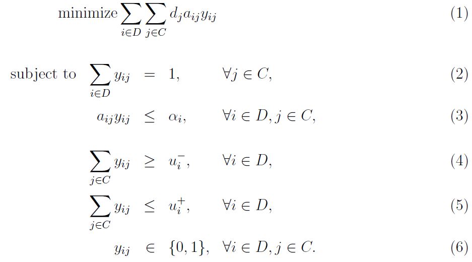
The objective of the model $(1)$ minimizes the total weighted distance. Constraint $(2)$ ensures that each customer is allocated to a center. There exists a maximum distance can be covered by each center $(3)$. Each center has minimum and maximum number of allocated customers as in $(4)$ and $(5)$, respectively. Center to customer allocation is binaries as in $(6)$.

Implementation

The algorithm is implemented in Python. Google OR Tools is used to solve the allocation problem.

You can find the source code at the Greenfield_With_Weighted_Kmeans repository on GitHub.

Application

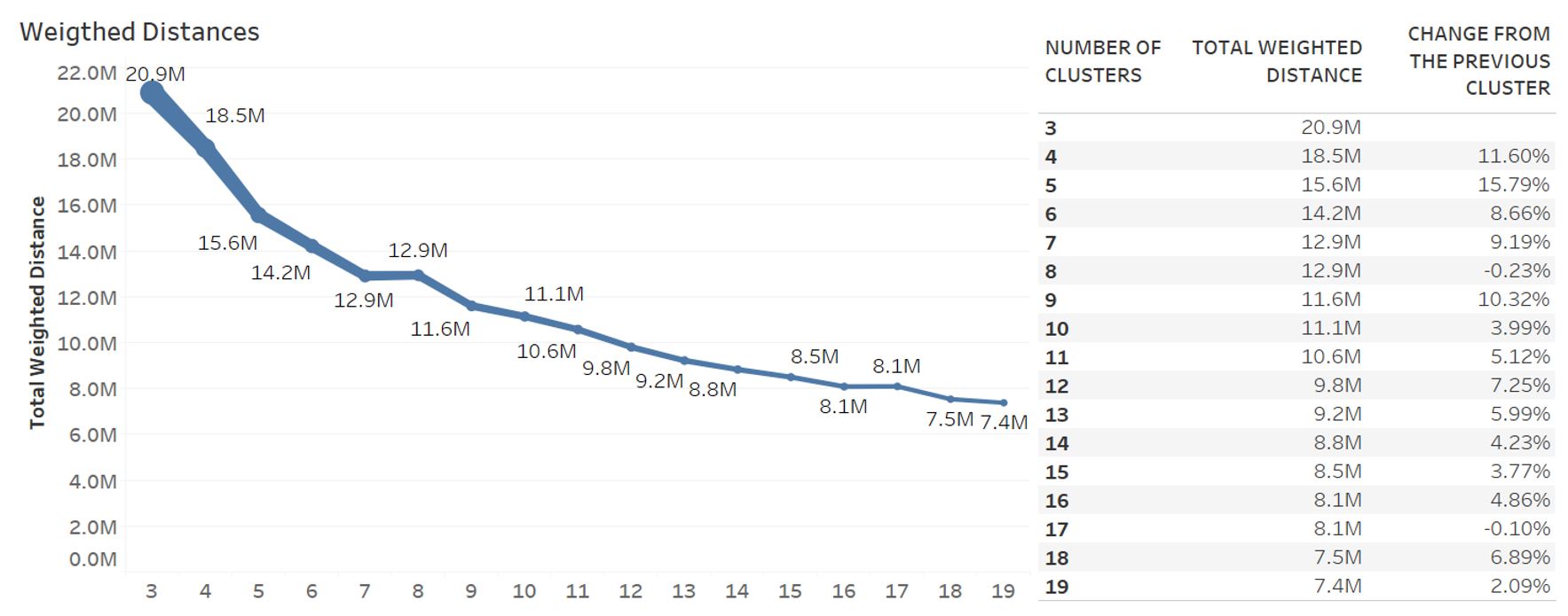
The algorithm is applied on the given problem. We iterate the algorithm for $n=3,\dots,19$. Figure 2 shows run results.

Figure 2: Results for $n=3,\dots,19$

Total weighted distance decreases as the number of clusters increases. More specifically, From $n=3$ to $n=7$, the total weighted distance is reduced by 39%. We find that $n=9$ is the best configuration since objective function improves slightly for $n>9$ and opening a new distribution center is costly.

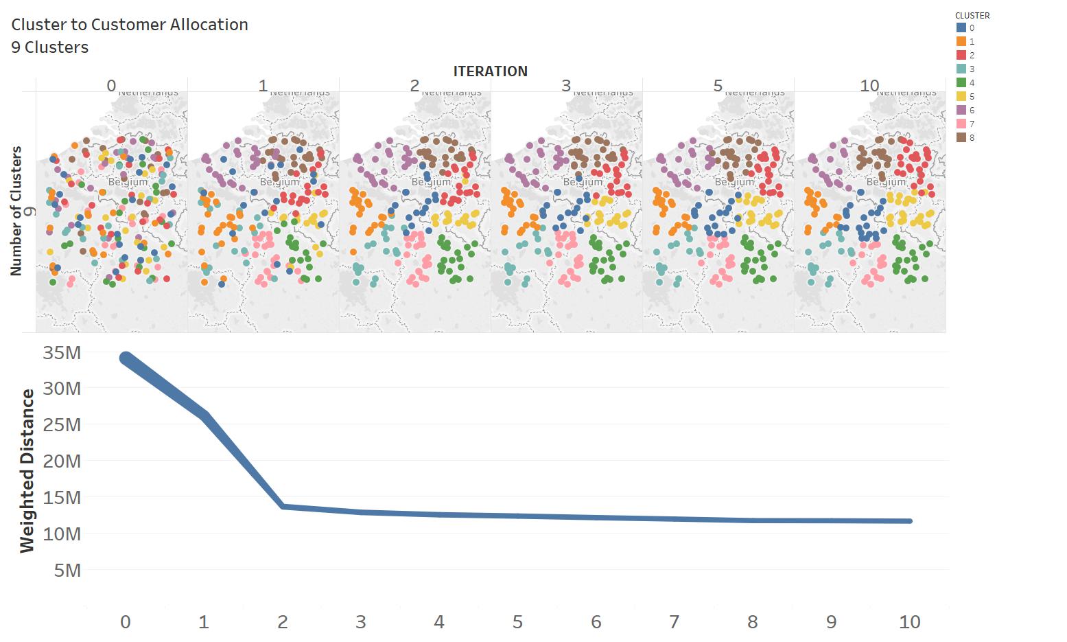
Figure 3 shows iteration steps for $n=9$. Algorithm converges quickly in the first three iterations and the total weighted distance reduces by $62\%$.

Figure 3: Algorithm iterations for $n=9$

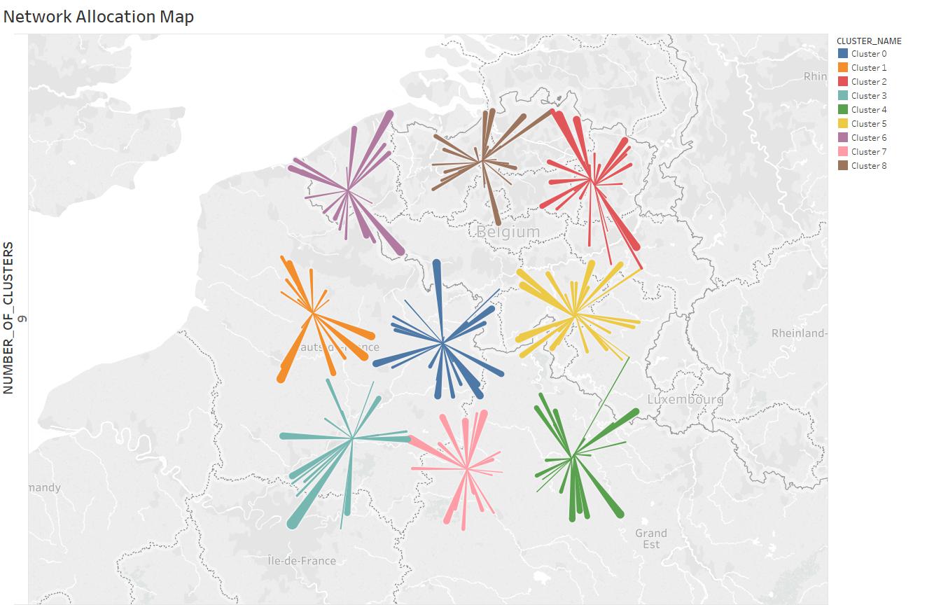
Allocation of customers to distribution centers is shown in Figure 4 for $n=9$ and $k=10$. Each distribution center covers customers in average $300$ miles radius.

Figure 4: Optimal flow map for $n=9$ and $k=10$

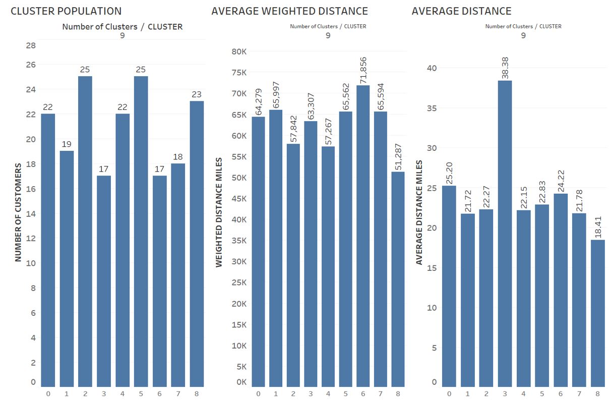
Figure 5 shows cluster statistics for $n=9$. We bound cluster size as $\mp$ 20% of average cluster size which is minimum $16$ and maximum $25$ for $n=9$. Cluster 8 average weighted distance is the lowest among all other clusters as well as the average distance.

Figure 5: Cluster statistics for $n=9$

Future Work

The Algorithm can be generalized to start with given $\hat{D}_i$ $\forall i\in D$ instead of creating $\hat{D}_i$ randomly. This will help to improve solution quality as well as to cover broader network design problems than the greenfield analysis.