Predicting Short Term Trucking Rates with Random Forests

In this post, we present a random forest model to predict short term trucking rates using Python.

Transportation rates are driven by different modes of transportation (air, road, rail, and ocean). In this work, we focus on trucking related transportation modes, Full Truckload (FTL) and Less than Truckload (LTL). We describe FTL and LTL modes, trailer types, and transportation services as follows.

FTL: An entire truck is used for transportation. In the FTL market, truck delivers to destination directly from shipper’s location using a dedicated truck. The rate is the same for the use of the full truck whether the truck is 100% full or 25% full and may be different depending on where the shipment starts and ends. Capacity of a truck can be measured in total weight, total cube, or total number of pallets. Various truck types are used such as regular dry van, refrigerated, flatbed, tanker, and 48- and 53-foot trailers. An FTL carrier may hold 45,000 pounds of product.

LTL: Companies use LTL when they have a small load to ship to a destination. In this case, hiring an entire truck to make the delivery is not economical. Trucking company picks up the load, combines it with other companies’ pickup or deliveries, and makes the trip to complete a route of deliveries to customer locations. An LTL carrier may hold up to 15,000 pounds of product.

Trailer Types: Different trailer types carry different products. The main types include dry van, flatbed, refrigerated/temperature-controlled trailer, and tank. Dry van is the most popular one. The flatbed trailer does not have a side wall or ceiling and used to carry construction materials or large machinery. Food and medicines are normally hauled by temperature-controlled. Tanks are used to haul refined oil products or chemicals in the liquid form.

Transportation Services: Two types of services exists to cover freight transportation requirements, through long-term contracts or on the spot market. Contract carriers is used most frequently. The contract is typically a one-year commitment, which consists of origin/destination, service requirement, volume and any other factors that affect the price. Spot market is used to obtain a rate when there is no availability in the contract market (lane does not exists or rate is not accepted).

Problem

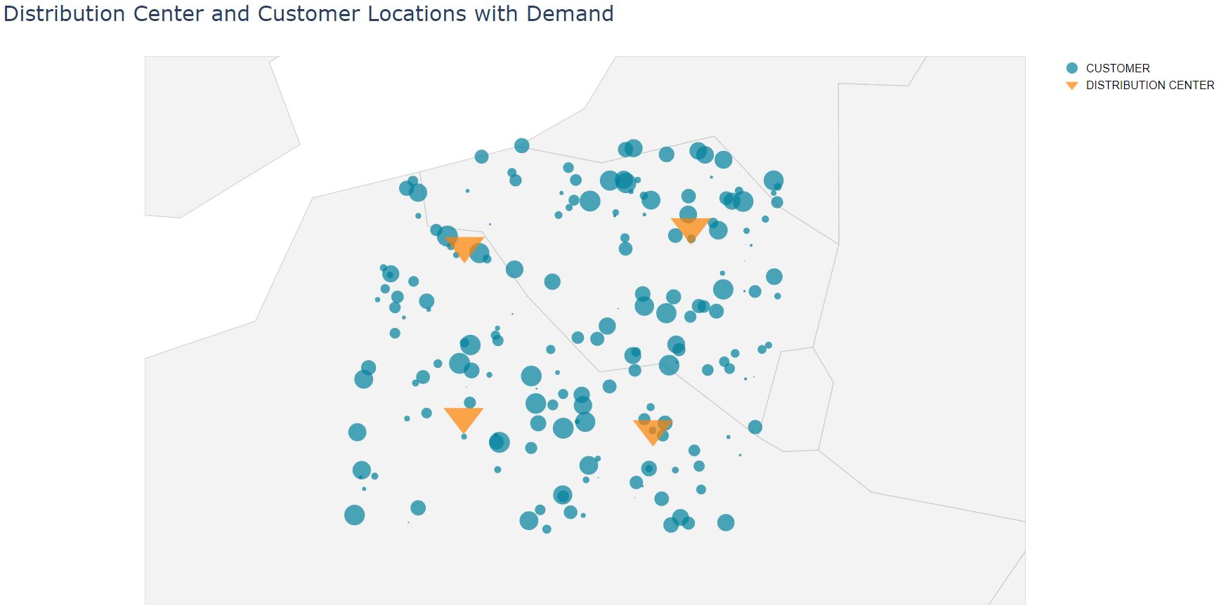
Consider a network of customers and distribution centers (see Figure 1). Products are delivered from distribution centers to customers using trucks.

Figure 1: Distribution centers and customers

Our objective is to determine FTL and LTL rates for each distribution center to each customer. We develop a model to predict transportation rates.

Analysis

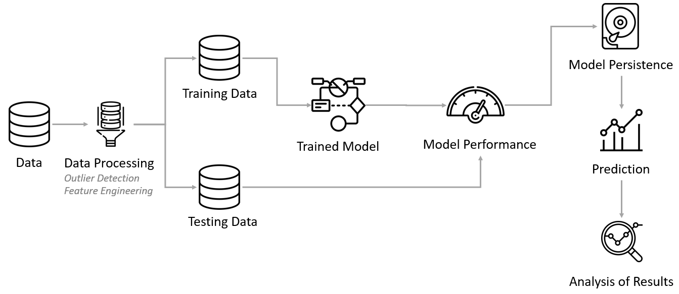
The following are the steps in the analysis, summarized by Figure 2.

1. Clean data, remove outliers
2. Create features (feature engineering)
3. Create train and test data
4. Develop model baseline
5. Fit model and measure performance
6. Interpret model and report results
7. Persist model

Figure 2: Analysis steps

We now explain each analysis step as follows.

1. Clean Data

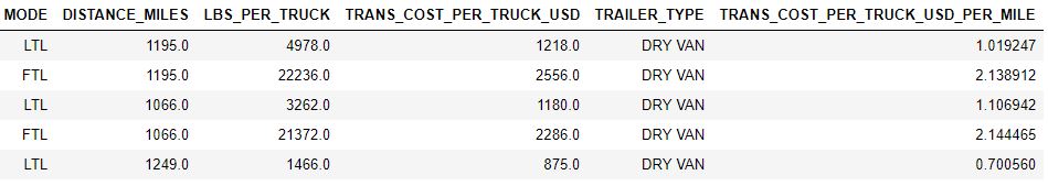
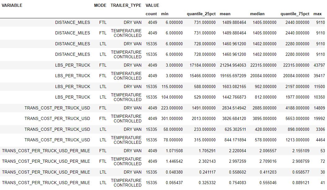
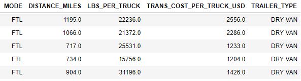
The dataset consists of the European long-haul Truckload data, including mode, distance covered per shipment, average shipment weight per truck, average shipment cost per truck, and trailer type (see Figure 3).

Figure 3: Transportation data set

Figure 4 shows the transportation data profiling by distance miles, average shipment per truck, transportation cost per truck, mode, and trailer type. We provide statistics by number of data points, minimum value, 25% quantile, mean, median, 75% quantile, and maximum value. The following Python code can be used to generate those statistics.

Figure 4: Transportation data set profile

def quantile_25pct(x):
    '''
    Get 25% quantile
    '''
    return x.quantile(0.25)

def quantile_75pct(x):
    '''
    Get 75% quantile
    '''
    return x.quantile(0.75)

trans_costs_melted.groupby(['VARIABLE', 'MODE', 'TRAILER_TYPE'], as_index=False).agg({'VALUE': ['count', 'min', quantile_25pct, 'mean', 'median', quantile_75pct, 'max']})

We fist analyze relationships between distance miles, shipment weight per truck, transportation cost per truck, and transportation cost per truck per mile for each mode and trailer. Then, we identify and remove outliers from the data set. The interquartile range (IQR) rule is applied to be able to detect outliers.

The following python functions are used to generate plots and to detect outliers.

import seaborn as sns

def plot_scatter(figure_data, x_axis_column, y_axis_column, legend_column, fig_width, fig_height, font_scale, grid_column, grid_row=None):
    '''
    Create a scatter plot
    '''
    sns.set(font_scale=font_scale)
    sns.set_style("white")
    if grid_row is None:
        g = sns.FacetGrid(figure_data, col=grid_column, hue=legend_column)
    else:
        g = sns.FacetGrid(figure_data, col=grid_column, row=grid_row, hue=legend_column)
    g = (g.map(sns.scatterplot, x_axis_column, y_axis_column, edgecolor="w").add_legend())
    g.fig.set_size_inches(fig_width, fig_height)

import numpy as np

def detect_outlier(data):
    '''
    Detect outliers using the IQR rule
    '''
    Q1 = data.quantile(0.25)
    Q3 = data.quantile(0.75)
    IQR = Q3 - Q1
    
    outliers = np.full(len(data), False)
    outliers[data < (Q1 - 1.5 * IQR)] = True
    outliers[data > (Q3 + 1.5 * IQR)] = True
    
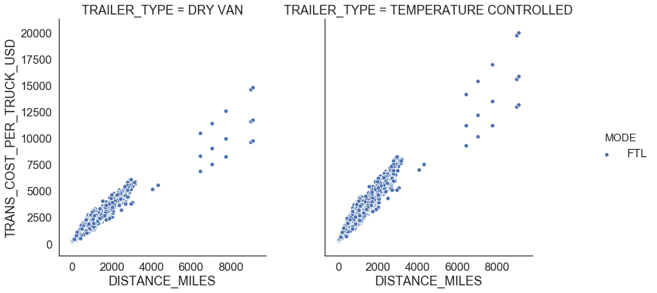
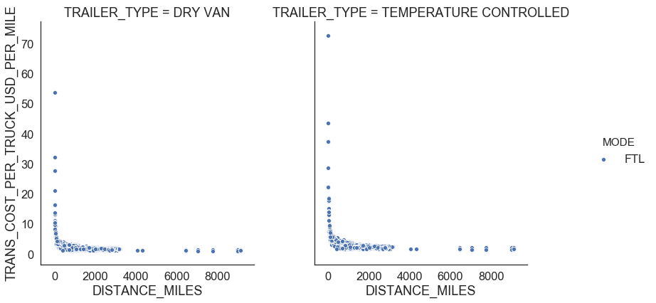
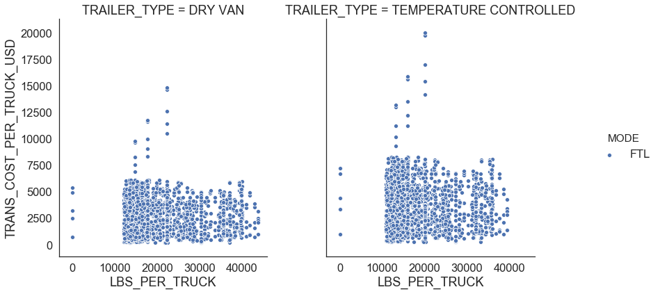
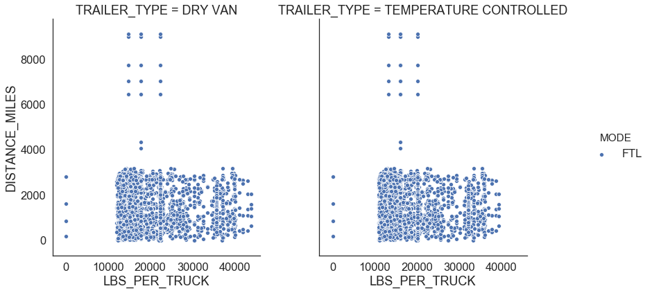
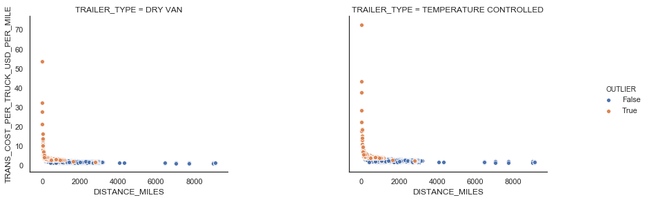
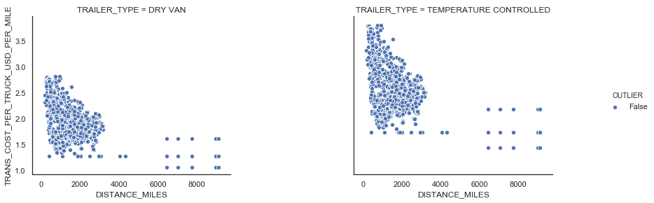
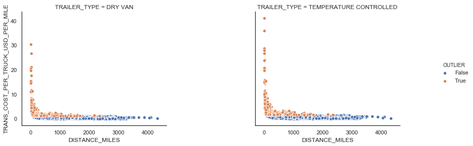
    return outliers

Figure 5 shows relationships for FTL. We observe that there is a linear relationship between distance traveled and transportation cost per truck which means that he FTL rate is the same whether the truck is 100% full or 25% full and changes depending on where the shipment starts and ends. We also see that FTL shipments in temperature controlled trailers are $0.7 more expensive per mile than the shipments in dry van (Figure 4).

Figure 5: FTL profiles

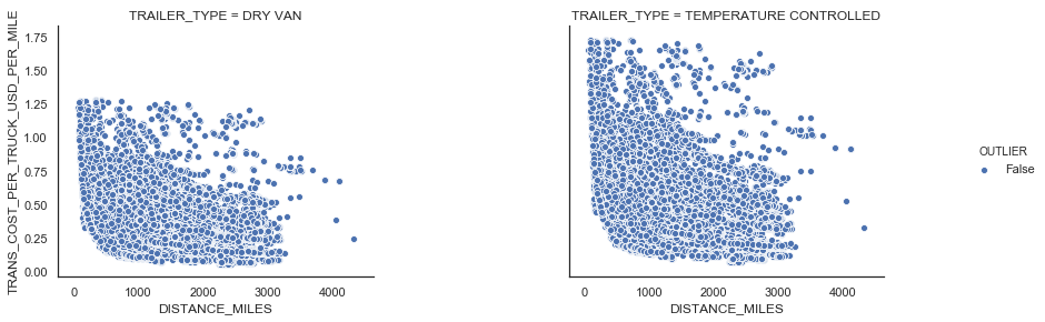
There are FTL shipments where shipment weight per truck is less than 10,000 LBS. We also identified points with a large transportation cost per truck per mile using the IQR rule. We consider those points as outliers and remove from the data set (see Figure 6).

Figure 6: FTL outliers

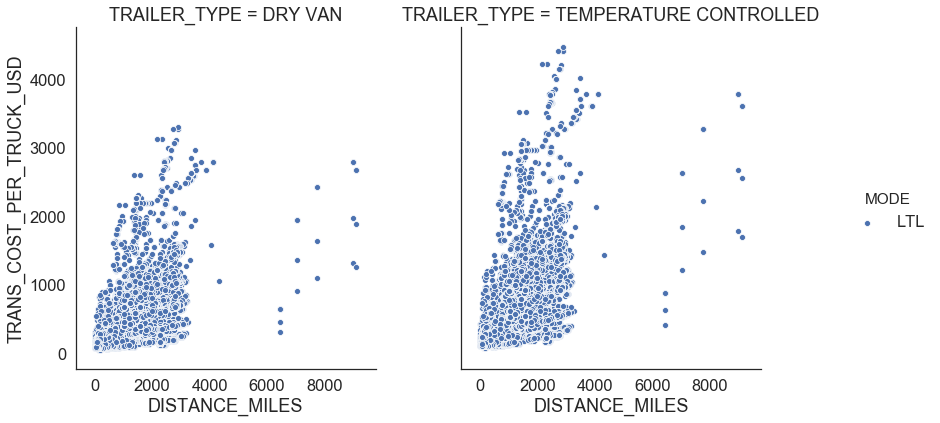
Figure 7 shows relationships between distance miles, shipment weight per truck, transportation cost per truck, and transportation cost per truck per mile for LTL. There is no clear distinct relationship between any of those variables.

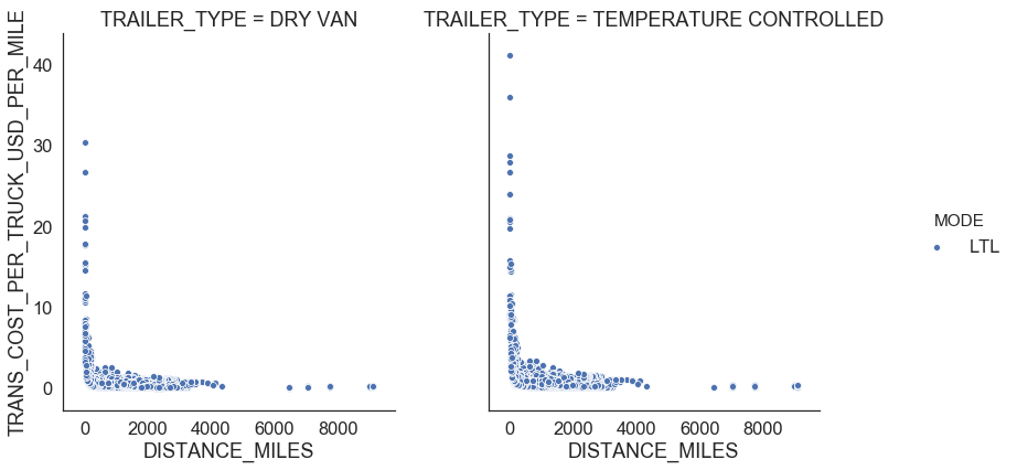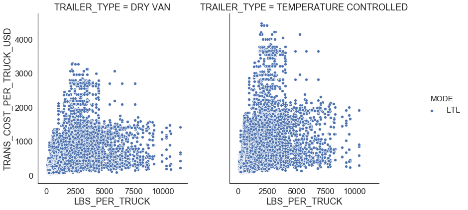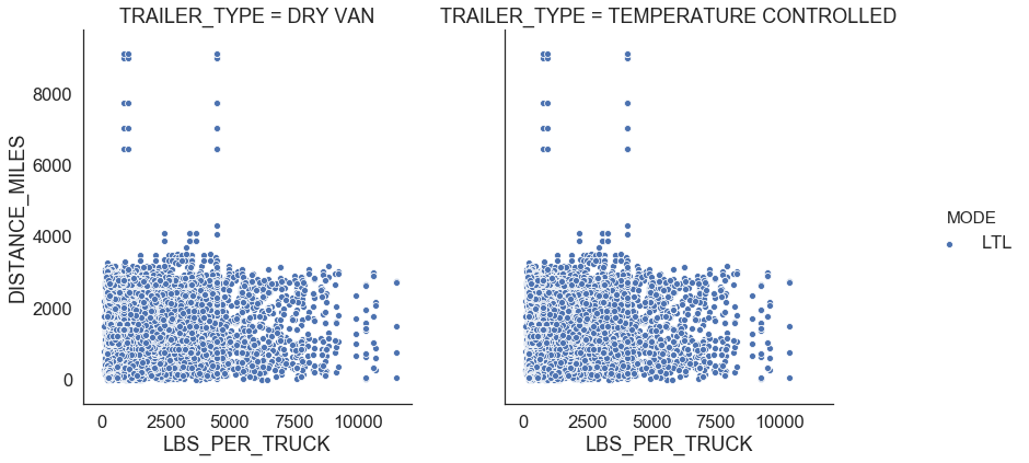Figure 7: LTL profiles

We treat shipments more than 5,000 mile distance as outliers since firms prefer FTL shipments for long distance since it is more economical comparing to LTL. After removing outlier points, we see a clear relationship between distance miles and transportation cost per truck for LTL (Figure 8).

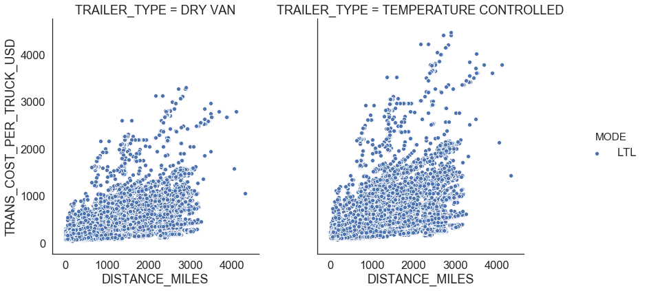Figure 8: LTL outliers

Similar in FTL, there exists LTL shipments with a large transportation cost per mile. We use the IQR rule to detect those outliers (see Figure 9).

Figure 9: LTL outliers

2. Create Features (Feature Engineering)

Feature engineering is the process of using domain knowledge of the data to create features for machine learning algorithms.

We use one-hot encoding to convert categorical data into a numerical format without losing any information. Figure 10 shows how FTL data is transformed as an example. We also provide Python code below for one-hot encoding.

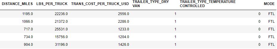Figure 10: FTL one-hot encoding

import pandas as pd

trans_cost_ftl_with_one_hot = pd.get_dummies(trans_cost_ftl.drop(['MODE', 'OUTLIER', 'TRANS_COST_PER_TRUCK_USD_PER_MILE'], 1))

3. Create Train and Test Data

At this step, we split data into training and testing sets to evaluate performance of the model. We randomly select 75% of the data for training and 25% of data for testing using the following Python function.

from sklearn.model_selection import train_test_split

def create_train_test_splits(labels_data, features_data, test_size):
    '''
    Create train and test data
    '''
    labels = np.array(labels_data)
    features_list = list(features_data.columns)
    features = np.array(features_data)

    train_features, test_features, train_labels, test_labels = train_test_split(features, labels, test_size = test_size, random_state = 42)

    return train_features, test_features, train_labels, test_labels

4. Develop Model Baseline

Before making predictions, we need to develop a model baseline to level set performance of the model. If the model can not improve the baseline, we need to try a new model.

In our problem, we set the baseline prediction as the average transportation cost per mile by mode and trailer type. We calculate Mean Absolute Error (MAE), Mean Percentage Error (MAPE), and accuracy as performance metrics.

We now define MAE, MAPE, and accuracy. Let $y_i$ be the prediction and $x_i$ be the actual value for $i=1, \dots, n$.

$$MAE = \frac{1}{n}\sum_{i=1}^n|y_i-x_i|$$ $$MAPE = 100\frac{1}{n}\sum_{i=1}^n\frac{|y_i-x_i|}{x_i}$$ $$Accuracy = 100 - MAPE$$

The following Python code is used to calculate baseline and accuracy metrics.

 
def apply_baseline_and_calculate_performance(trans_cost_with_one_hot, test_features, features_list, test_labels):
    '''
    Calculate baseline
    '''
    baseline = trans_cost_with_one_hot.groupby(['MODE', 'TRAILER_TYPE_DRY VAN', 'TRAILER_TYPE_TEMPERATURE CONTROLLED'], as_index=False).agg({'TRANS_COST_PER_TRUCK_USD': 'sum', 'DISTANCE_MILES': 'sum'})
    baseline['TRANS_COST_PER_TRUCK_USD_PER_MILE'] = baseline['TRANS_COST_PER_TRUCK_USD'] / baseline['DISTANCE_MILES']
    baseline.drop(['DISTANCE_MILES'], 1, inplace=True)
    
    baseline_costs = pd.DataFrame(test_features)
    baseline_costs.columns = features_list
    
    baseline_costs = baseline_costs.merge(baseline, how='left', on=['TRAILER_TYPE_DRY VAN', 'TRAILER_TYPE_TEMPERATURE CONTROLLED'])
    baseline_costs['BASELINE_TRANS_COST_PER_TRUCK_USD'] = baseline_costs['DISTANCE_MILES'] * baseline_costs['TRANS_COST_PER_TRUCK_USD_PER_MILE']
    baseline_costs['ACTUAL_TRANS_COST_PER_TRUCK_USD'] = test_labels
    baseline_costs['ABSOLUTE_ERROR'] = abs(baseline_costs['BASELINE_TRANS_COST_PER_TRUCK_USD'] - baseline_costs['ACTUAL_TRANS_COST_PER_TRUCK_USD'])
    baseline_costs['MAPE_PCT'] = 100 * (baseline_costs['ABSOLUTE_ERROR'] / baseline_costs['ACTUAL_TRANS_COST_PER_TRUCK_USD'])
    
    mean_absolute_error = round(np.mean(baseline_costs['ABSOLUTE_ERROR']), 2)
    accuracy = round(100 - np.mean(baseline_costs['MAPE_PCT']), 2)
    
    return baseline_costs, mean_absolute_error, accuracy

We calculate baseline performance metrics for FTL and LTL is as follows. Those provide us goals which is model performance should be better than baseline performance.

	FTL Baseline	LTL Baseline
MAE	434.46	352.96
MAPE	12.38%	66.9%
Accuracy	87.62%	33.1%

5. Fit Model and Measure Performance

We use the train data to fit the random forest model and the test data to measure model performance. We calculate MAE, MAPE, and Accuracy similar to the baseline analysis.

The following functions are used to fit the random forest model and measure the model performance.

 
from sklearn.ensemble import RandomForestRegressor

def fit_random_forest_model(train_features, train_labels):
    '''
    Fit a random forest model
    '''
    random_forest = RandomForestRegressor(n_estimators = 1000, random_state = 42)
    random_forest.fit(train_features, train_labels)
    return random_forest

def prediction_and_metrics(random_forest, test_features, test_labels):
    '''
    Predict and measure the model performantce
    '''
    predictions = random_forest.predict(test_features)
    
    mae = round(np.mean(abs(predictions - test_labels)))
    mape = np.mean(100 * (mae / test_labels))
    accuracy = 100 - np.mean(mape)
    
    return predictions, mae, mape, accuracy

The following table provides baseline and random forest model performance metrics for FTL and LTL.

	FTL Baseline	LTL Baseline	FTL Random Forest Model	LTL Random Forest Model
MAE	434.46	352.96	188.0	123.0
MAPE	12.38%	66.9%	7.12%	33.10%
Accuracy	87.62%	33.1%	92.88%	66.90%

Both FLT and LTL models beat the baseline prediction. FTL model prediction has 94% accuracy. However,
LTL model’s accuracy is 67% which is lower than FTL model.

One way to improve LTL model’s performance is hyperparameter tuning where the model settings are adjusted to improve performance. Another way is to add more features to the data set to capture behavior better.

6. Interpret Model and Report Results

We can use two methods to be able to understand how model calculates the values,

1. Visualizing a random forest tree
2. Understanding feature importance of variables

Visualizing A Random Forest Tree

The following Python code is used to visualize one of the random forest trees in the model.

 
from IPython.display import SVG
from graphviz import Source
from sklearn.tree import export_graphviz 

def create_random_forest_tree_image(random_forest_model, tree_number, features_list, tree_file_name):
   '''
   Create and save random forest tree image
   '''
    tree_in_forest = random_forest_model.estimators_[tree_number]
    graph = Source(export_graphviz(tree_in_forest, out_file=None
       , feature_names=features_list
       , filled = True))

    png_bytes = graph.pipe(format='png')
    with open('{}.png'.format(tree_file_name),'wb') as f:
        f.write(png_bytes)
        
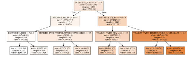
    return 'tree is created'

Figure 11 shows one of the random forest trees in the model. Since the tree is very large, it is hard to visualize the relationships between model variables.

Figure 11: Random forest tree

We limit maximum depth to be 3 to be able to visualize a tree (see Figure 12).

Figure 12: Random forest tree where maximum depth = 3

Let’s assume that we want to predict transportation cost per shipment with the following shipment features.

Mode	Trailer Type	Weight Load (LBS)	Shipment Distance (Miles)
FTL	Dry Van	17,404	341

We follow the path in Figure 13 and predict FTL transportation cost per shipment as $1,277.

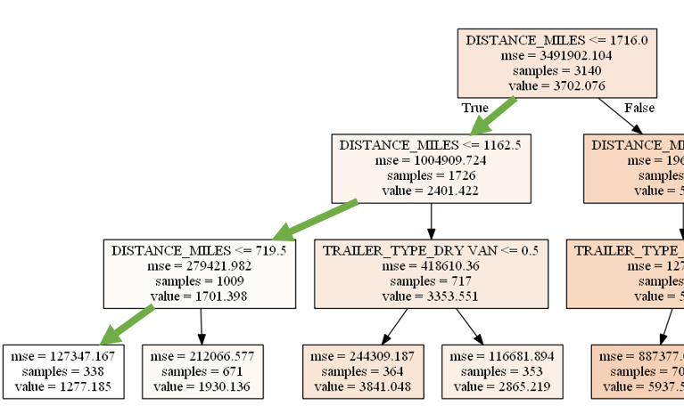Figure 13: Predicting for FTL rate for a Dry Van, 341 miles distance, and 17,404 LBS weight with the model where maximum depth = 3

Understanding Feature Importance of Variables

The relative importance is defined as how much including a particular variable improves the prediction. We use the following code to calculate importance of model variables.

 
def calculate_feature_importance(random_forest_model, feature_list):
    '''
    Calculate feature importance
    '''
    importances = list(random_forest_model.feature_importances_)
    feature_importances = [(feature, round(importance, 2)) for feature, importance in zip(feature_list, importances)]
    feature_importances = sorted(feature_importances, key = lambda x: x[1], reverse = True)
    
    feature_importances = pd.DataFrame(feature_importances)
    feature_importances.columns = ['FEATURE', 'IMPORTANCE']
    
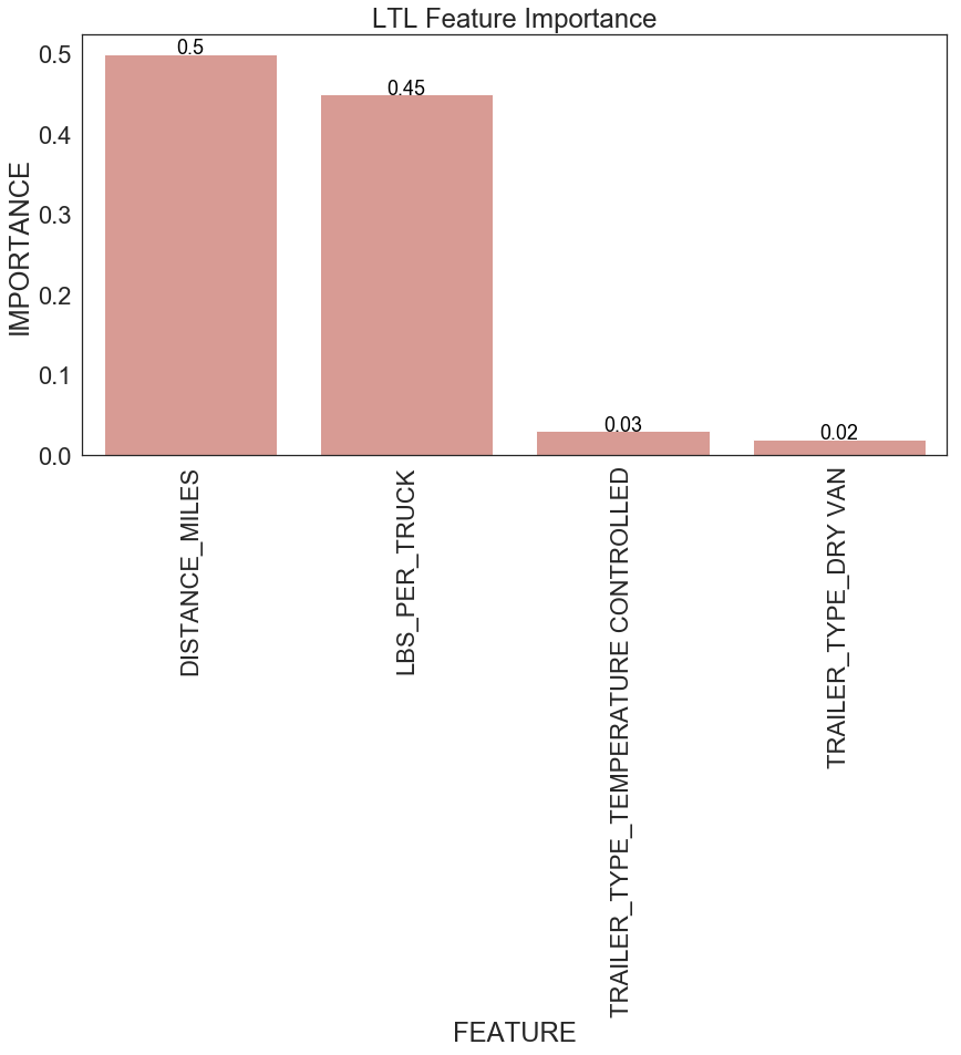
    return feature_importances

Figure 14 shows feature importance for FTL and LTL. For FTL, miles travelled is the most important factor for predicting transportation cost per shipment. This is aligned with the observation we have before (see Figure 5). Miles travelled and weight per shipment are the two most important variables affecting transportation cost per shipment for LTL.

Figure 14: Feature importance for FLT and LTL

7. Persist Model

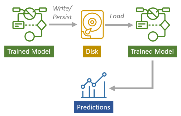
Model persistence is a technique where trained model is written or persisted to the disk. And once you have your model saved on the disk, you can use it whenever you want. After you read and load the file and get the trained model back that you can use for making predictions. This is a very powerful technique because now you don’t have to train the model every time in order to use the trained model. You can persist your trained model once, and then you can use it later. You can also share your training model with others without sharing the training data and all of the steps to train the model (see Figure 15).

Figure 15: Model persistence

We use the following Python code to persist the random forest model.

 
import pickle

def persist_model(random_forest_model, feature_list, train_features, train_labels, test_features, test_labels, filename):
    '''
    Persist model
    '''
    tuple_objects = (random_forest_model, feature_list, train_features, train_labels, test_features, test_labels)
    pickle.dump(tuple_objects, open(filename, 'wb'))
    return 'model saved to '.format(filename)

We load the saved model using the following Python function.

 
def load_model(filename):
    '''
    Load persisted model
    '''
    random_forest_model, feature_list, train_features, train_labels, test_features, test_labels = pickle.load(open(filename, 'rb'))
    return random_forest_model, feature_list, train_features, train_labels, test_features, test_labels